Traditional parametric models, characterized by a fixed and finite number of parameters, can encounter issues of data overfitting or underfitting when there is a mismatch between the model’s complexity (often represented by the parameter count), the complexity of the true data generation process, and the available data volume. Consequently, it frequently becomes necessary to engage in model selection to identify the most suitable model from a variety of potential options. Regrettably, model selection is a demanding and laborious task, irrespective of whether frequentist cross-validation or Bayesian marginal probabilities are employed as the selection criteria.
The Bayesian nonparametric (BNP) approach presents an alternative to parametric modeling and selection. It adapts its complexity according to the available data quantity or the complexity of the data generation process. This inherent flexibility helps mitigate underfitting, while the Bayesian methodology for computing complete posteriors addresses the issue of overfitting. It’s worth noting that we refer to a model as parametric when it possesses a finite number of parameters, whereas a nonparametric model assumes, a priori, an infinite number of parameters.
In the context of Bayesian nonparametric models, a BNP model defines a probability distribution across an infinite-dimensional parameter space. While this might initially seem intricate, in practice, a BNP model employs only a finite subset of the potentially infinite parameters to explain any finite set of observations.
Mixture models
Finite mixture models
Let’s start with a straightforward parametric model frequently employed for clustering or density estimation purposes: The Gaussian Mixture model.
We can express the generative model for $K$ clusters as follows:
\[\mu_k \sim \mathcal{N}(\mu_0, \Sigma_0)\] \[\pi \sim Dir(\alpha)\] \[z_n \sim Cat(\pi)\] \[x_n \sim \mathcal{N}(\mu_{z_n},\Sigma)\]Here, $\mu_k$ represents the cluster means, with one for each of the $K$ clusters. Conversely, $z_n$ signifies the cluster memberships, and $\pi$ denotes the mixing coefficients.
For any finite set of $N$ observations, $x_n \in \mathbb{R}^d$, the model encompasses $N + Kd + K - 1$ parameters, encompassing the cluster memberships, cluster means, and mixing coefficients. Thus, we indeed categorize it as parametric. It’s worth noting that there are additional hyperparameters, namely the priors’ parameters $\mu_0, \Sigma_0, \alpha, \Sigma$. For simplicity, let’s set $\mu_0 = 0$ and $\Sigma_0 = I$, which makes sense if we standardize the data. Additionally, we’ll assume $\Sigma=0.1I$. However, selecting a suitable value for $\alpha$ presents a challenge. What impact does $\alpha$ have? You can explore this question in the plot below.
As evident from the generative model, $\alpha$ influences the mixing coefficients $\pi$. As $\alpha$ approaches 0, the Dirichlet distribution concentrates at the corners of the unit simplex, indicating a scenario with a few dominant clusters and many small ones. Conversely, as $\alpha$ increases towards infinity, the distribution converges to a point mass at $1/K$.
Now, for any observed dataset $X$, we can infer the parameters using Bayes’ theorem:
\[p(Z, \pi, \mu_{1:K}\mid X) \propto p(X\mid \mu_{1:K},Z)p(Z\mid \pi)p(\pi)p(\mu_{1:K}) = \prod_{n=1}^N \mathcal{N}(x_n; \mu_{z_n}, 0.1I)Cat(z_n;\pi)Dir(\pi;\alpha) \prod_{k=1}^K \mathcal{N}(\mu_k;0,I)\]Although a closed-form solution is not attainable, we can employ MCMC methods like Gibbs Sampling to sample from it.
Unfortunately, this model has one limitation. If the data requires more than $K$ cluster centers, then we have a problem. Hence we have to do model selection i.e. we have to choose the best $K$. Intuitively, we shouldn’t need more clusters than number of data points we observe, right? Not necessarily, just imagine there are 1000 latent components and we observe only 100 data points then we cannot observe more than 100 clusters, right?
So let’s look what will happen if we sequentially observe one datapoint $x_i$ at a time. There are two events that can happen:
- $x_i$ can be part of a cluster we already observed.
- $x_i$ can be part of a new cluster.
Let’s say we have $K=1000$ components. How many points do we need to observe all 1000 components? At which rate do we observe new components? As always try to answer the question yourself, the animation below will help by simulation this process.
Letting $K \rightarrow \infty$ now seems less unreasonable, doesn’t it? After all, we will ultimately observe a finite number of observations, leading to only a finite number of components! Keep in mind that the simulation above employs $K = 1000,” so the line will eventually flatten as we approach 1000 (though you might need to wait forever for that :D). In the next section, we will delve into how we can set $K = \infty$.”
The Stickbreaking construction
The primary challenge we encounter when letting $K \rightarrow \infty$ is the potential for the Dirichlet distribution to become ill-defined. After all, how can we sample a vector of infinite length? At a certain point at least your memory will say goodbye!
As is often the case, the solution lies in laziness! In the simulation mentioned earlier, even after observing a thousand data points, we only observed 200 clusters. So, instead of sampling mixture coefficients for all potentially infinite components, we can opt for a more efficient approach. We can lazily generate a new component only when it becomes necessary. Let’s consider $K=2$ and an alternative method to sample from a Dirichlet distribution is to utilize the Beta distribution.
\[\pi_1 = \mathcal{B}(\alpha_1, \alpha_2) \quad \text{ and } \quad \pi_2 = 1-\pi_1\]It’s quite straightforward to observe that $(\pi_1, \pi_2) \sim \text{Dir}((\alpha_1,\alpha_2))$, as we can deduce from the fact that the marginal distribution of a Dirichlet is always a Beta distribution. Now, let’s extend this concept to an arbitrary value of $K$, which is commonly referred to as Stickbreaking.
Imagine we have a stick of length 1, representing the total probability mass. Our objective is to break this stick into $K$ pieces. By definition, these pieces must collectively sum to one. We initiate this process as follows:
- Draw $\phi_1 \sim \mathcal{B}(\alpha_1, \sum_{k=2}^K \alpha_k)$. Set $\pi_1 = \phi_1$ and break a part of lenght $\pi$ from the stick.
- Draw $\phi_2 \sim \mathcal{B}(\alpha_2, \sum_{k=3}^K \alpha_k)$. The remaining stick has length $(1-\pi_1)$, thus break of a part of length $\pi_2 = \phi_2(1-\pi_1)$.
- …
- Draw $\phi_i \sim \mathcal{B}\left(\alpha_i, \sum_{k=i+1}^K \alpha_k\right)$. Set $\pi_i = \prod_{j=1}^{K-1}(1-\phi_j) \phi_i = \phi_i \cdot \left(1-\sum_{j=1}^{i-1}\pi_i\right)$
- …
- Set $\pi_K = 1- \sum_{k=1}^{K-1}\pi_k$.
This approach allows us to efficiently generate a sequential series of $K$ numbers that collectively sum to one. However, the question arises: why did we limit ourselves to just $K$ pieces? Is it possible to extend this process indefinitely?
As it turns out, this concept is (almost) accurate; we can, in fact, generalize the method outlined above:
- Draw $\phi_1 \sim \mathcal{B}(a_1, b_1)$. Set $\pi_1 = \phi_1$.
- Draw $\phi_2 \sim \mathcal{B}(a_2, b_2)$. Set $\pi_2 = (1-\phi_1)\phi_2$
- …
- Draw $\phi_i \sim \mathcal{B}(a_i,b_i)$. Set $\pi_i = \prod_{j=1}^{K-1}(1-\phi_j) \phi_i$
- …
In this manner, we generate an infinite sequence $\pi_1, \pi_2, \dots$, from which we can, at least, ensure that $\sum_{k=1}^\infty \pi_k \leq 1$. But, hold on, why doesn’t it equal one?
This discrepancy becomes apparent through a counterexample. Consider the sequence $\pi_i = 1/(2^n+2)$. In this case, $\sum_{i=1}^\infty \pi_i = 1/2 \leq 1$. Hence, we need to ensure that we cannot sample such sequences, or at the very least, that the probability of sampling them is zero (the set of such sequences should have negligible measure). Interestingly, it is possible to achieve this by constraining the set of parameters $a_i, b_i$ within the process (as outlined in Ishwaran and James, 2001). In practice, convergence to a finite sum typically occurs quite swiftly, and the process is often truncated after a certain point. Regardless, at some stage, floating-point precision may pose an issue. You can explore this for yourself here:
It appears that if we select $a_1=1$ and $\beta = \alpha > 0$, then with a probability of 1, all sequences we sample will ultimately converge to 1. This is precisely what we need. We now refer to this underlying process as the Dirichlet process stick-breaking, and the underlying distribution is known as the GEM distribution. Once again, we can examine the number of observed “clusters.” If you were to allow the animation below an infinite amount of time, you would indeed see it approaching infinity. However, in contrast to the previous plot, the only limiting factors here are your finite time and memory capacity…
Infinite mixture models
After discovering the GEM distribution, we can now easily write up a generative model for a mixture model with an infinite number of components.
\[\pi = (\pi_1, \pi_2, \dots) \sim GEM(\alpha)\] \[\mu_k \sim \mathcal{N}(\mu_0, \Sigma_0) \text{ for } k=1,2, \dots\] \[z_n \sim Cat(\pi)\] \[x_n \sim \mathcal{N}(\mu_{z_n}, \Sigma)\]Now, let’s examine some samples from this process. It’s important to note that we cannot sample it in its entirety since doing so would demand an infinite amount of time and memory. However, we can generate data sequentially, much like we did previously! In the animation below, you can experiment with this process, particularly exploring the influence of a single hyperparameter, $\alpha$, on the number of clusters we would actually observe in a finite dataset. It’s essential to keep in mind that while all the samples theoretically possess an infinite number of components, practical constraints like finite time and memory prevent us from observing all of them ;)
Dirichlet process: Formal definition
Let $\Theta$ represent a parameter space, and let $G_0$ be a base measure defined over $\Theta$. Once again, we draw $\pi \sim GEM(\alpha)$ and $\theta_k \sim G_0$. Consequently, we refer to $G = \sum_{k=1}^\infty \pi_k \delta_{\theta_k}$ as a draw from a Dirichlet process (DP), denoted as $G \sim DP(\alpha, G_0)$. Here, $\delta_{\theta_k}$ signifies an indicator function applied to a specific $\theta_k$ sampled from the base measure. Thus, every draw from a DP embodies this infinite object. We can regain the previous scenario by simply setting $\Theta = \mathbb{R}^2$ and $G_0 = \mathcal{N}(\mu_0, \Sigma_0)$. In this context, all the $\theta_k$ now correspond to an infinite number of potential cluster centers, each associated with a specific mixing coefficient $\pi_k$.
In fact, these objects $G$ have a specific property. They are measures over the parameter space $\Theta$ (in fact even a probability measure!). To see that consider some set $A \subset \Theta$ then \(G(A) = \sum_{k=1}^\infty \pi_k \delta_{\theta_k}(A) = \sum_{k: \theta_k \in A} \pi_k\) So in fact the DP is a distribution over random measures.
The nomenclature may prompt some inquiries: Why is it referred to as a Dirichlet process? What attributes qualify it as a stochastic process, an assemblage of indexed random variables? Furthermore, how does it relate to the Dirichlet distribution? Do its random variables conform to a Dirichlet distribution? And what exactly constitutes the index set? To illuminate this, let’s begin with a predefined set $A \subset \Theta$. Is it correct to regard $G(A)$ as a random variable? The answer lies in the inherent randomness of $G$ itself. Indeed, by its very construction, we observe that $G(A) \in [0,1]$, resembling a typical marginal sample extracted from a Dirichlet distribution. To delve deeper, we can investigate $B = \Theta \backslash A$, wherein we ascertain that, by construction, $G(A) + G(B) = 1$. This prompts the consideration of the random vector $(G(A), G(B))$. Given that any realized instance of this vector must sum to one, it bears a striking resemblance to a draw from a Dirichlet distribution. But what governs its parameters? Intuitively, it appears to be proportionate to the volume of $A$ under the base measure $G_0$. This suggests that if $A$ encompasses a substantial portion of the support provided by $G_0$, most indicator functions must reside within it. Remarkably, this intuition aligns with reality, as it turns out that $(G(A), G(B)) \sim Dirichlet((\alpha G_0(A), \alpha G_0(B)))$ (Here the details). Thus, we have established that a partition of $\Theta$ into $A$ and $B$ generates a random vector distributed according to a Dirichlet distribution. Notably, this holds true for any finite partition of $\Theta$. Consequently, we have identified the index set of this stochastic process as encompassing all possible partitions of $\Theta$. This newfound clarity enables us to formally define this process as follows:
In essence, the Dirichlet Process (DP) embodies a stochastic process that delineates a distribution over distributions, specifically probability measures. Each draw from a DP inherently embodies a distribution. Its nomenclature, “Dirichlet process,” stems from its possession of Dirichlet-distributed finite-dimensional marginal distributions, akin to the Gaussian process—a widely employed stochastic process in Bayesian nonparametric regression. It’s worth noting that distributions drawn from a DP are not only discrete but also infinite in nature.
As a consequence, an alternative representation of the Dirichlet Process Mixture Model can be articulated as follows:
\[G \sim DP(\alpha, \mathcal{N}(\mu_0, \Sigma_0))\] \[\mu_k \sim G\] \[x_n \sim \mathcal{N}(\mu_k, \Sigma)\]Note that we no longer require to use the latent variables $z_n$ i.e. the cluster memberships.
The Dirichlet process posterior
Consider $G \sim DP(\alpha, G_0)$. As $G$ represents a random distribution itself, we can draw samples $\theta_1, \dots, \theta_n \sim G$. It’s essential to note that the $\theta_i’s$ assume values within the set $\Theta$ since $G$ is a distribution over $\Theta$. Now, let’s assume our interest lies in the posterior distribution of $G$ after observing $\theta_1, \dots, \theta_n$.
Let $A_1, \dots, A_r$ constitute a finite measurable partition of $\Theta$. Define $n_k$ as the count of observed values falling within $A_k$, expressed as $n_k = \sum_{i=1}^n I(\theta_i \in A_k)$. By leveraging the conjugacy between the Dirichlet and multinomial distributions, we deduce the following: \((G(A_1,), \dots, G(A_r)) \mid \theta_1, \dots, \theta_n \sim Dir(\alpha G_0(A_1) + n_1, \dots, \alpha G_0(A_r) + n_r)\) Since this holds true for all finite measurable partitions, the posterior distribution over $G$ retains the form of a Dirichlet Process, as all its marginals continue to be Dirichlet-distributed. The question then arises: How should we adjust the parameters? To address this query, let’s examine our initial definition:
You can verify easily that for any finite partition, we obtain a Dirichlet posterior distribution as derived above.
Notice that we can rewrite the posterior as following \(G\mid \theta_1, \dots,\theta_n \sim DP\left(\alpha + N, \frac{\alpha}{\alpha + N} G_0 + \frac{N}{\alpha + N} \frac{\sum_{i=1}^N \delta_{\theta_i}}{n}\right)\) Hence, the posterior emerges as a composite distribution, blending the base distribution $G_0$ and the empirical distribution. The weight attributed to the base distribution scales proportionally with $\alpha$, whereas the empirical distribution carries a weight proportional to the count of observations, denoted as $N$. Consequently, we can interpret $\alpha$ as the mass assigned to the prior. As $\alpha \rightarrow 0$, the prior tends towards non-informativeness, signifying that the predictive distribution is solely governed by the empirical distribution.You can play with the posterior distribution in the below animation. You can add observations by just taping into the figure with your mouse (a red dot will appear!). At this moment you condition our previous prior on this particular observation. You can look at multiple samples for different alpha and verify the above intuition we build up.
Note: We draw the means from the DP and within the above simulation we do condition the means $\mu_k$, not the observation $x$. We will come to the second case latter.
The predictive distribution and the Chinese restaurant process
Let’s revisit the scenario where $G$ follows a Dirichlet Process, denoted as $G \sim DP(\alpha, G_0)$, and we draw an independent and identically distributed (i.i.d.) sequence $\theta_1, \theta_2, \dots \sim G$. Now, consider the predictive distribution for $\theta_{n+1}$, conditioned on $\theta_1, \dots, \theta_n$, with $G$ integrated out.
Due to conditional independence, $\theta_{n+1}\mid G, \theta_1, \dots, \theta_n \sim G$, implying that $\theta_{n+1}$ is independent of $\theta_1, \dots, \theta_n$ given $G$. Therefore, we have: \(P(\theta_{n+1} \in A \mid \theta_1, \dots, \theta_n) = \mathbb{E}\left[ G(A) \mid \theta_1, \dots, \theta_N \right] = \frac{1}{\alpha + N} \left( \alpha G_0(A) + \sum_{i=1}^N \delta_{\theta_i}(A) \right)\) Consequently, with $G$ integrated out, we find that: \(\theta_{N+1}\mid \theta_1, \dots, \theta_N \sim \frac{\alpha G_0 + \sum_{i=1}^N \delta_{\theta_i}}{\alpha + N}\)
This reveals that the posterior base measure coincides with the predictive distribution. This alignment allows us to draw samples according to the following scheme:
- With probability $\frac{\alpha}{\alpha + N}$ draw $\theta_{N+1} \sim G_0$
- Else draw some $\theta_1, …, \theta_N$ uniformly.
The Chinese Restaurant Process serves as a metaphorical description of this generative model. In this metaphor, customers enter a Chinese restaurant equipped with an infinite number of tables. The first customer selects the initial table. Subsequently, each new customer decides to either join an existing table or open a new one. In general, the $(n+1)$-th customer can select from one of the $K$ occupied tables with a probability proportional to the number of customers already seated there or initiate a new table with a probability proportional to the concentration parameter $\alpha$.
It’s worth noting that the earlier-described simulation faithfully adheres to this process.
Applications
In this section, we will delve into practical and useful applications.
Infinite mixture models
Let’s apply our acquired knowledge to a real-world dataset of tweets from former US President Donald Trump, which you can access on Github).
Our primary objective is to identify a collection of topics that Donald Trump was interested in during and after his presidency. Here, we define a topic as a set of keywords, and we categorize a tweet into a specific topic if it contains a significant number of relevant keywords. Since we lack prior knowledge about the exact number of topics, we can make the a priori assumption of an infinite number of potential topics.
The dataset presents certain complexities, comprising natural language and various Twitter-specific artifacts such as retweets (which are not authored by Donald Trump and should be excluded from our analysis). However, our focus is solely on extracting topics, so we can streamline the tweets by distilling them into a list of specific keywords. This process results in a more straightforward tweet2vec embedding. Each vector within this embedding corresponds to a predefined keyword dictionary (I’ve chosen 400 keywords), and it encodes the frequency of each keyword’s occurrence within the tweet.
With these simplifications in place, we can formulate a relatively straightforward generative model for this dataset:
\[G \sim DP(\alpha, Dir(\gamma))\] \[\theta_k \sim G\] \[x_n \sim Cat(\theta_k)\]In contrast to the previous examples, our approach now incorporates a Dirichlet Base measure since we are dealing with Categorical data, specifically a bag of words representation. While we’ve been sampling from the posterior distribution of a Dirichlet Process conditioned on $\theta_k$, we must now introduce a Categorical likelihood component since we observe the data vector $x_n$. Without delving into the intricacies here, it’s worth noting that there are various methods to handle this, such as employing Gibbs sampling.
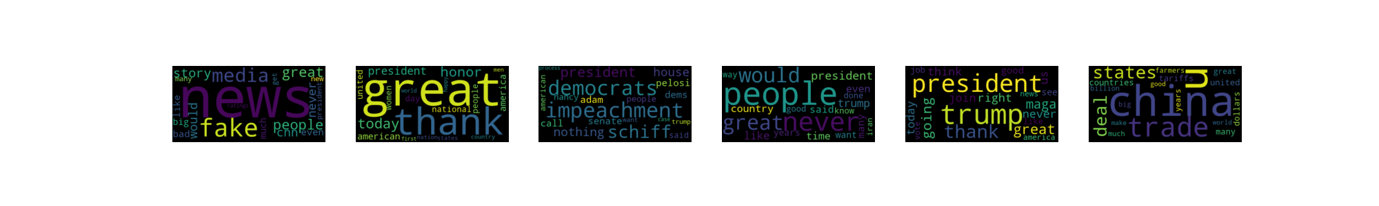
The outcomes of this approach are indeed intriguing. Below, you’ll find word clouds that illustrate the top eight “Trump Twitter topics” that we’ve uncovered through our analysis. These word clouds provide a visual representation of the most frequently occurring keywords within each topic, offering valuable insights into the content of Donald Trump’s tweets.
Bayesian bootstrap inference
Whereas the last example (and most of this post) got an fully Bayesian treatment we for now we want to draw a little inspiration from the dark side: Let’s forget the posterior as ultimate goal of inference for a moment.
Imagine that our observations are samples drawn from an unknown generative process: $x_1, \dots, x_n \sim \mathbb{P}^\star$. We posit that this process can be expressed as $\mathbb{P}^\star = p_{\theta^\star}$, where $\theta^\star$ represents an elusive and unknown parameter. This concept isn’t entirely novel and aligns with the prerequisites of a well-specified Bayesian model.
In Bayesian inference, we would typically assign a prior distribution to $\theta$ and compute the posterior distribution, denoted as $p(\theta \mid x_{1:n})$. It’s evident that the posterior should concentrate its density around values of $\theta$ in the vicinity of $\theta^\star$, in harmony with our prior beliefs. However, it’s essential to recognize that, for any finite number of observations (assuming appropriate priors and likelihoods), the posterior will exhibit a degree of uncertainty regarding the true value of $\theta^\star.
For a moment let’s assume we know $\mathbb{P}^\star$, then inference on $\theta^\star$ is easy. We just solve e.g.
\[\theta^\star = \arg \min_{\theta} D_{KL}(P^\star \mid \mid p_\theta) = \arg \min_{\theta} \mathbb{E}_{P^\star}\left[ -\log p_\theta(x)\right].\]No uncertainty about $\theta^\star$ arises! Yet in practice we typically do not have access $P^\star$, put only a set of i.i.d. observations i.e. an empirical approximation \(\mathbb{P}_n = \frac{1}{n} \sum_{i=1}^n \delta_{x_i}\). We still can try to recover $\theta^\star$ by solving
\[\hat{\theta} = \arg \min_{\theta} -\frac{1}{N}\sum_{i=1}^N \log p_\theta(x_i).\]Which leads to the maximum likelihood estimator. Yet, different $\mathbb{P}_n^{(i)}$ lead to different estimates $\hat{\theta}^{(i)}$, so which $\hat{\theta}^{(i)}$ should we trust? Which one is closest to $\theta^\star$? Fundamentally uncertainty arises every time as long $N < \infty$. So despite no Bayesian treatment, we again arrive at some distribution over $\theta$ … (it’s not the same as the posterior, but is very related known as a bootstrap distribution).
Yet to sample from this distribution we require a number of independent datasets of size $N$ i.e. \(\mathbb{P}_n^{(1)}, \dots, \mathbb{P}_N^{(m)}\) , which is even harder than before. In frequentist statistics there is a simple but efficient approximation, known as bootstrap estimates. There we typically start with a single dataset \(\mathbb{P}_N\). Then just subsample it $m$ time i.e. \(\mathbb{P}_N^{(j)} = \frac{1}{n}\sum_{i=1}^n \delta_{x_i}\) for \(x_i \sim \mathbb{P}_N\). It is easy to see that this is a good approximation only if $N » n$. So let’s try to be a bit more Bayesian.
We just learned that we can efficiently compute posterior on a distribution over distributions! Thus if we don’t know $P^\star$, but have some observations $x_1, \dots, x_N \sim \mathbb{P}^\star$, then why shouldn’t we just infer the posterior over $\mathbb{P}^\star$. If we choose an Dirchlet process prior on it, then as we saw the posterior is closed from and computationally efficient. As a result we then can sample from a “bootstrap posterior” over $\theta$ by just sampling $\mathbb{P}^{(j)} \sim \mathbb{P}\mid x_1, \dots, x_N$. Instead of an empirical estimate we now can estimate $\theta^\star_{(j)}$ exactly given $\mathbb{P}^{(j)}$.
Let’s consider a easy example. Consider the true generative process \(\mathbb{P}^\star = \mathcal{N}(x; \theta^\star, \sigma^2).\) We are interested in estimating $\theta^\star$. Our prior over it is a Dirichlet process i.e.
\[DP(\alpha, G_0) \qquad \text{ with } G_0 = \mathcal{N}(0, 1)\]We condition the prior on data and obtain the posterior
\[\mathbb{P}\mid x_1, \dots, x_n \sim DP\left(\alpha + N, \frac{\alpha}{\alpha + N} G_0 + \frac{N}{\alpha + N} \frac{\sum_{i=1}^N \delta_{x_i}}{n}\right)\]We thus can get samples $\mathbb{P}^{(j)} \sim \mathbb{P}\mid x_1, \dots, x_n$ from which we know it has the form \(\mathbb{P}^{(j)} = \sum_{k=1}^\infty \pi_k \delta_{x_k}\)
We obtain that
\[\theta^\star = \arg \min_\theta D_{KL}(\mathbb{P}^{(j)}\mid \mathcal{N}(x; \theta, 1)) = \arg \min_\theta - \sum_{k=1}^\infty \pi_k \log p_\theta(x_k)\] \[= \arg \min_\theta \sum_{k=1}^\infty \pi_k (x_k - \theta)^2\]Diverentiating with respect to $\theta$ we get
\[\nabla_\theta \sum_{k=1}^\infty \pi_k (x_k - \theta)^2 = 2 \sum_{k=1}^\infty \pi_k \theta - 2 \sum_{k=1}^\infty \pi_k x_k \iff \theta^\star_{(j)} = \sum_{k=1}^\infty \pi_k x_k\]And that’s all. Sounds complicated. Sounds wierd, but is surprisingly easy to implemenet. You can test it here:
You can play around a bit with the “hyperparameters” i.e. $\alpha$ and the base measure $G_0$.
Leave a Comment