All about Fisher information

Fischer information plays a pivotal role in statistics; as we will see in some way or another, it will pop up in both Frequentist and Bayesian statistical paradigms. In this post, I will introduce the Fisher information together with some essential properties. We will review several applications and relationships of the Fischer information to other important quantities.

Notation and Definition

Suppose we have a parametric statistical model $p_{\theta}(x)$ with parameter vector $\theta$ modeling some distribution. We aim to learn an unknown distribution $p(x)$ from which we have i.i.d. samples $x_1, \dots, x_N \sim p(x)$. In frequentist statistics, the most common approach to learn $\theta$ is by maximizing the likelihood $\prod_{i=1}^N p_\theta(x_i)$ with respect to the parameter $\theta$. To assess the goodness of fit, we can use the so-called (Fischer) score, which we define as

\[s_x(\theta) = \nabla_\theta \log p_\theta(x).\]

To justify this as a measure of goodness, consider the following claim:

[theorem] Be $\log p_\theta(x)$ differentiable in $\theta$ almost everywhere and let the support of $p_\theta$ be independent of $\theta$. Then it holds that \(\mathbb{E}_{p_\theta(x)} \left[s_x(\theta)\right] = \mathbb{E}_{p_\theta(x)} \left[ \nabla_\theta \log p_\theta(x)\right] = 0\) [/theorem] [proof] As we can interchange integration and differentiation under the above regularity conditions, it holds that \(\begin{aligned}\mathbb{E}_{p_\theta(x)} \left[ \nabla_\theta \log p_\theta(x)\right] &= \int \frac{\nabla_\theta p_\theta(x)}{p_\theta(x)} p_\theta(x)dx \\ &= \int \nabla_\theta q (x)dx \\&= \nabla_\theta \int p_\theta(x)dx \\&= \nabla_\theta 1\\& = 0 \end{aligned}\) [/proof]

Thus, assuming we found some nice estimator $\theta^*$, we would expect that if it is a good fit, we have that

\[\mathbb{E}_{p(x)}\left[ s_{x}(\theta)\right] \approx \frac{1}{N} \sum_{i=1}^N \nabla_{\theta^*} \log p_{\theta^*}(x_i) \approx 0.\]

Indeed, as $N \rightarrow \infty$, this tends toward zero if and only if $p_{\theta^*} = p$! However, our primary concern lies in measuring deviations from zero to assess the goodness of fit. This brings us to the central theme of this post: The Fisher information (matrix).

(Fisher information): Assuming the score $s(\theta)$ has a bounded second moment under $p_\theta$, then the Fisher information (matrix) is defined as $$F(\theta) := \Sigma_{q} \left( s_x(\theta) \right) = \mathbb{E}_{p_\theta(x)} \left[ s_x(\theta)s_x(\theta)^T \right]$$

We can again approximate the expectation of the empirical data distribution, yielding the empirical Fisher $\hat{F}(\theta)$, that can again be evaluate at our selected parameter $\theta$

\[\hat{F}(\theta) = \frac{1}{N} \sum_{i=1}^N s_{x_i}(\theta) s_{x_i}(\theta)^T\]

It’s important to note that this estimate captures the deviation of the score from zero, rather than from the actual mean. The mean is only zero when $p = p_\theta$. Therefore, this estimate remains unbiased only when $x_i \sim p_\theta$. In any scenario, high Fisher information indicates that the absolute value of the score tends to be large.

A quick look at wikipedia gives us the following intuitive definition

"In mathematical statistics, the Fisher information is a way of measuring the amount of information that an observable random variable $X$ carries about an unknown parameter $\theta$ of a distribution that models X."

So, let’s go through some examples

Example 1: Bernoulli model

Let’s consider a coin-flip experiment. The coin $X$ will be distributed according to a Bernoulli distribution.

\[Ber(x;\theta) = \theta^X (1-\theta)^{1-X}\]

Given $N$ observations $x_1, \dots, x_N \sim Ber(x;\theta)$, we can denote the loglikelihood as

\[\log p(X|\theta) = \sum_{i=1}^N \log p(x_i|\theta) = (\sum_{i=1}^N x_i)\log \theta + (N - \sum_{i=1}^N x_i) \log (1-\theta)\]

Thus, let’s first derive the score function of this problem.

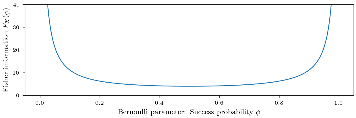
\[s_X(\theta) = \nabla_\theta \log p(X|\theta) = \frac{(\sum_{i=1}^N x_i)}{\theta} - \frac{(N - \sum_{i=1}^N x_i)}{1-\theta} = \frac{\sum_{i=1}^N x_i (1-\theta) - N\theta + \sum_{i=1}^N x_i \theta}{\theta(1-\theta)} = \frac{\sum_{i=1}^N x_i - N\theta}{\theta (1-\theta)}\]

Notice that the score is zero if the sum of Bernoulli trials equals the expected i.e. $N\theta$, a consequence of Theorem 1. Furthermore, the magnitude of the score is determined by $1/(\theta (1-\theta))$, which is minimized if $\theta=0.5$ and approaches infinity for $\theta \rightarrow 1$ and $\theta \rightarrow 0$. As a result, changes within the parameter near zero or one will lead to a large score! Recall that the score equals the gradient of the log-likelihood. A large score thus indicates that small changes within the parameter can strongly change the log-likelihood.

So let’s compute the corresponding Fisher information, as we defined it before

\[F(\theta) = \mathbb{E}_{p_\theta(x)} \left[ s(\theta)^2) \right] = \frac{\mathbb{E}_{p_\theta(x)} \left[ (\sum_{i=1}^N x_i - N\theta)^2 \right] }{\theta^2 (1-\theta)^2} = \frac{Var_{p_\theta(x)} \left( \sum_{i=1}^N x_i\right) }{\theta^2 (1-\theta)^2} = \frac{N \theta (1-\theta)}{\theta^2 (1-\theta)^2} = \frac{N}{\theta (1-\theta)}\]

Indeed, the Fisher information exhibits intriguing properties. Firstly, it linearly increases with the number of considered data points. This aligns with the intuition that more independent and identically distributed (i.i.d.) samples provide more insights about the unknown parameter. As we’ll explore later, this behavior is a universal trait. Secondly, it is inversely proportional to the variance of the distribution. This relationship makes sense since we can glean more information about the unknown parameter from random variables with smaller variances. However, it’s worth noting that this property’s generalizability isn’t as obvious as one might intuitively assume.

Example 2: Exponential family

Let’s look at a more general family, which also includes the previous example: The exponential family. Be $T(x)$ the sufficient statistics, $\eta$ the natural parameters, and $Z,h$ the partition function and the base measure. Then, an exponential family model is defined as

\[p_\eta (x) = h(x) \exp(\eta^T T(x) - Z(\eta))\]

with $Z(\eta) = \log \int h(x) \exp(\eta^TT(x)) dx$. The log-likelihood is thus for $N$ observations $x_1, …, x_N$ is thus given by

\[\log p_\eta(X) = \sum_{i=1}^N \eta^T T(x_i) - Z(\eta) + \log h(x_i)\]

For notational simplicity, let’s assume $N=1$, then the score of an exponential family is given by

\[s_x(\eta) = \nabla_\eta \log p_\eta(x) = T(x) - \nabla_\eta Z(eta)\]

Notice that by this and Theorem 1, it follows that $\mathbb{E}{p\eta}[T(x)] = \nabla_\eta Z(eta)$. A lovely property of the exponential family. Let’s get to the Fisher information.

\[F(\eta) = \mathbb{E}_{p_\eta} \left[ (T(x) - \nabla_\eta Z(eta))(T(x) - \nabla_\eta Z(eta))^T \right] = \Sigma_{p_\eta(x_i)}(T(x))\]

Thus the Fisher information equals the covariance of the sufficient statistic $T(x)$! But wait, the Bernoulli distribution is an exponential family, right? And we just calculated that the Fisher information equals the inverse variance in this case. So, isn’t this a contradiction?

No, we just discovered that Fisher information can change upon a change in parameterization. Remember, before, the parameter $\theta$ was the probability of success. In contrast, $\eta = \log \frac{\theta}{1 - \theta}$ gives the natural parameter for a Bernoulli distribution. But luckily, as we will later see, we can translate between different parameterizations relatively easy.

Properties of the Fisher information

If we observe i.i.d. samples, each sample should contain the same amount of information.

Be $X$ and $Y$ be two independent random variables, then $$ F_{X,Y}(\theta) = F_{X}(\theta) + F_{Y}(\theta)$$

[proof] We can write \(\begin{aligned} F_{X,Y}(\theta) &= \mathbb{E}_{X,Y}\left[ s_{X,Y}(\theta)s_{X,Y}(\theta)^T \right]\\ & = \int \int \nabla_\theta \log p(x,y|\theta) \left( \nabla_\theta \log p(x,y|\theta) \right)^T p(x)p(y)dxdy\\ &= \int \int \nabla_\theta (\log p(x|\theta) + \log p(y|\theta)) \left( \nabla_\theta (\log p(x|\theta) + \log p(y|\theta)) \right)^T p(x)p(y)dxdy\\ &= \int \nabla_\theta \log p(x|\theta)(\nabla_\theta \log p(x|\theta))^Tp(x) dx + \int \nabla_\theta \log p(y|\theta)(\nabla_\theta \log p(y|\theta))^Tp(y) dx\\ & \quad + \int \int \nabla_\theta \log p(x|\theta) (\nabla_\theta \log p(y|\theta))^T p(x)p(y)dxdy\\ & \quad + \int \int \nabla_\theta \log p(y|\theta) (\nabla_\theta \log p(x|\theta))^T p(y)p(x)dydx\\ &= \mathbb{E}_{X}[s_X(\theta) s_X(\theta)^T] + \mathbb{E}_{Y}[s_Y(\theta) s_Y(\theta)^T] + \int \underbrace{\mathbb{E}_X[ s_{X}(\theta)]}_{= 0} s_Y(\theta)^T p(y)dy + \int \underbrace{\mathbb{E}_Y[ s_{Y}(\theta)]}_{= 0} s_X(\theta)^T p(x)dx\\ & = F_X(\theta) + F_Y(\theta) \end{aligned}\) [/proof]

So this is great, and by it, we can easily explain how the Fisher information behaves under the i.i.d. assumption:

If $X_1, \dots, X_N$ are i.i.d. then $$ F_{X_1, \dots, X_n}(\theta) = N \cdot F_{X_1}(\theta)$$

We can extend Lemma 1 to a more general case where $X$ and $Y$ are not independent:

Be $X$ and $Y$ two random variables jointly distributed according to $p(X,Y)$. Then $$ F_{X,Y}(\theta) = F_{X|Y}(\theta) + F_Y(\theta) = F_{Y|X}(\theta) + F_X(\theta)$$ Where we define the conditional Fisher information as $$ F_{X|Y} = \mathbb{E}_Y\left[ F_{X|y = Y}(\theta) \right] = \mathbb{E}_Y\left[ \int \nabla_\theta \log p(x|y = Y) (\nabla_\theta \log p(x|y = Y))^T p(x|y=Y) \right]$$

[proof] As above just using the product rule $\log p(X,Y) = \log p(X|Y) + \log p(Y) = \log p(Y|X) + \log p(X)$ [/proof]

We already saw that the Fisher information depends on the parameterization of our statistical model. Let’s quantify exactly how different parameterizations do change the Fisher information.

Be f a totally differentiable map from parameter with $\eta = f(\theta)$, where both parameters encode the same statistical model. Be $J_f = \nabla_\theta f(\theta)$ the Jacobian matrix, then $$ F_{x}(\theta) = J_f^T F_X(f(\theta)) J_f $$

[proof] This simply follows from the chain rule of differentiation. Notice that we can write [\(\displaystyle \begin{aligned}s_x(\theta)= \nabla_\theta \log p_{f(\theta)}(x) = \nabla_\theta f(\theta) \nabla_\eta \log p_\eta(x) = J_f^T \nabla_\eta \log p_\eta(x) = J_f^T s_x(\eta) \end{aligned}\)
By the definition of Fisher information, we have that \(F_x(\theta) = \mathbb{E}_{p_\theta}\left[s_x(\theta)s_x(\theta)^T \right] = \mathbb{E}_{p_\theta}\left[J_f^Ts_x(\eta)s_x(\eta)^TJ_f \right] = J_f^T F_x(\eta) J_f\)
which completes the proof. [/proof]

Recall that the natural parameters of a Bernoulli distribution are $\eta = f(\theta) = \log \frac{\theta}{1-\theta}$. Thus $\nabla_\theta f(\theta) = \frac{1}{\theta(1-\theta)}$, we had that the Fisher information of an exponential family equals the covariance of the test statistic. For a Bernoulli variable, we thus have

\[F_x(\eta) = f^{-1}(\eta) (1- f^{-1}/\eta) = \theta (1-\theta)\]

Thus, by applying the above lemma, we get \(F_x(\theta) = \frac{\theta (1-\theta)}{(\theta (1-\theta)^2} = \frac{1}{\theta (1-\theta)}\) which is exactly what we obtained by explicitly calculating it.

Another beneficial property is the connection to the Hessian of the log-likelihood. This is often used as an alternative definition and can also simplify the computation.

Be $\log p_\theta(x)$ twice differentiable and be $H_{\log q (x)} = \nabla_\theta \nabla_\theta^T \log p_\theta(x)$ the corresponding Hessian. Then, it holds that $$ F_X(\theta) = -\mathbb{E}_{p_\theta (x)} \left[ H_{\log q (x)} \right]$$

[proof] We can write the Hessian of the log-likelihood as follows \(H_{\log q (x)}= \nabla_\theta \nabla_\theta^T \log q (x) = \nabla_\theta \frac{\nabla_\theta^T p_\theta(x)}{q (x)} = \frac{ \nabla_\theta \nabla_\theta^T q (x) p_\theta(x) - \nabla_\theta q (x) \nabla_\theta^T q (x)}{p_\theta(x)^2} = \frac{H_{ q (x)}}{q (x)} - \frac{\nabla_\theta q (x) \nabla_\theta^T q (x)}{q (x)^2}\)
Which simply follows from the chain and quotient rule of differentiation. Let’s apply the expectation to the first term. \(\mathbb{E}_{q (x)} \left[ \frac{H_{ q (x)}}{q (x)} \right] = \int H_{ q (x)} dx = \int \nabla_\theta \nabla_\theta^T q (x)dx = \nabla_\theta \nabla_\theta^T \int q (x) dx = \nabla_\theta \nabla_\theta^T 1 = 0\)
So this term vanishes, let’s apply it to the second term \(\mathbb{E}_{q (x)} \left[ - \frac{\nabla_\theta q (x) \nabla_\theta^T q (x)}{q (x)^2} \right] = - \mathbb{E}_{q (x)} \left[ \left( \frac{\nabla_\theta q (x)}{q (x)}\right) \left( \frac{\nabla_\theta q (x)}{q (x)}\right)^T \right] = - \mathbb{E}_{q (x)} \left[ \left( \nabla_\theta \log q (x)\right) \left( \nabla_\theta \log q (x)\right)^T \right]\)
which proves the statement. [/proof]

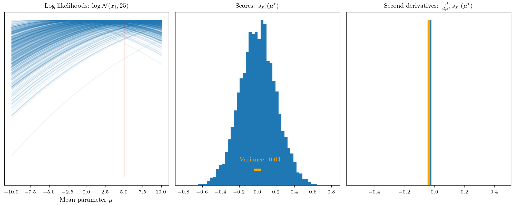
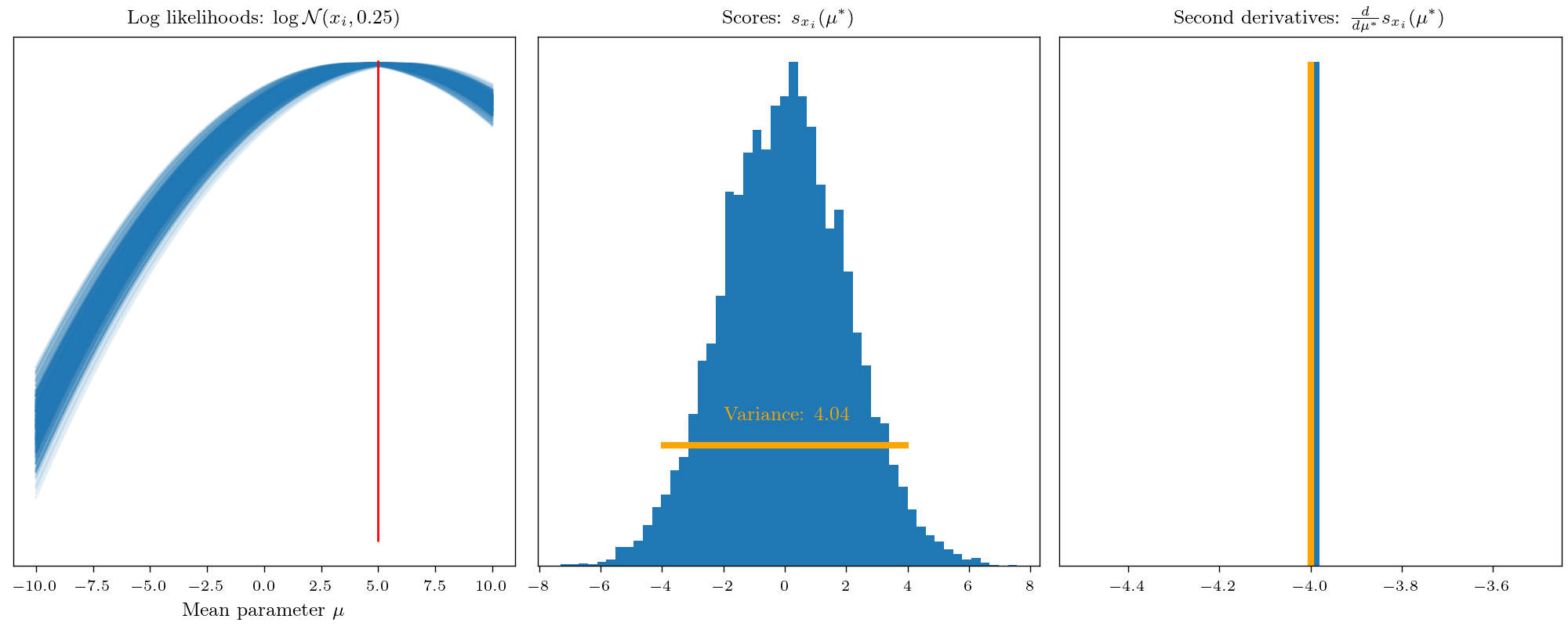
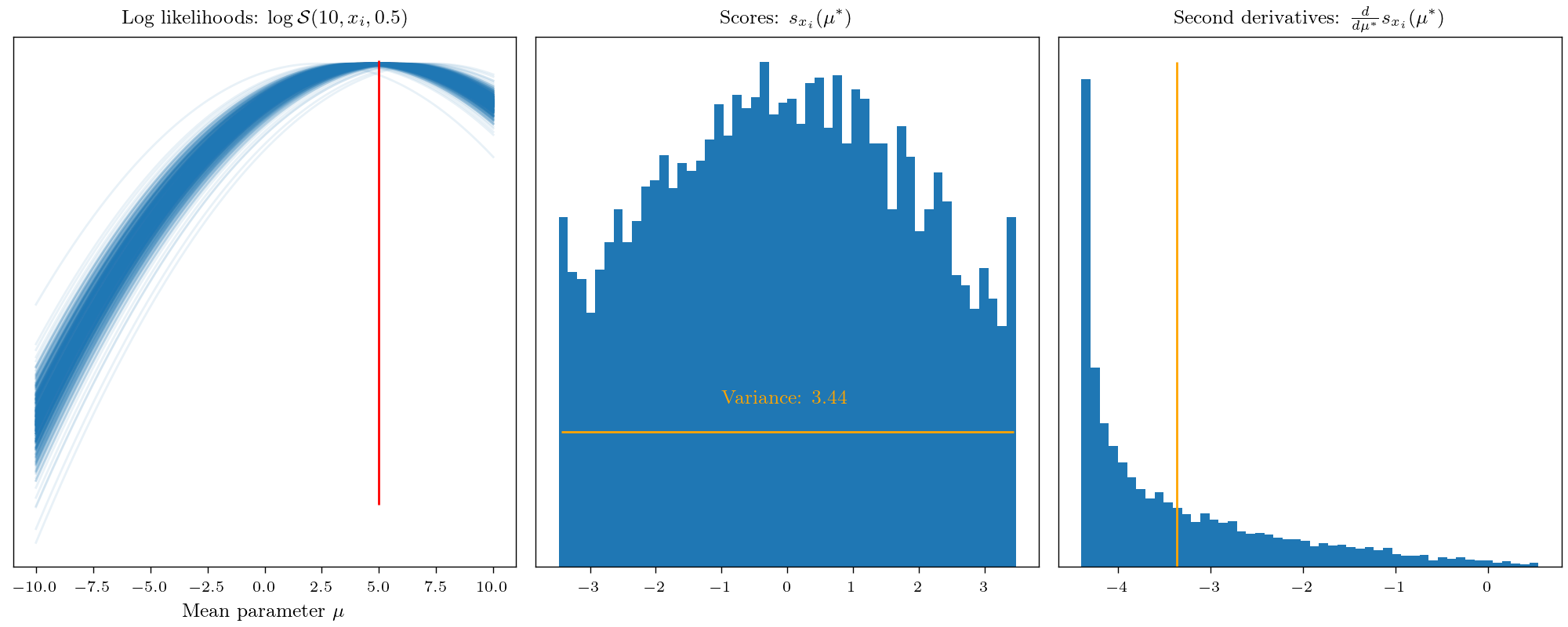
This allows interpreting the Fisher information as the average curvature of the log-likelihood. Low Fisher information implies that the likelihood function’s peaks are shallow, and neighboring values exhibit similar log-likelihoods. Conversely, high Fisher information indicates sharp peaks, where small parameter changes strongly affect the log-likelihood. To visualize this concept, let’s remember that the Fisher information represents how easily we can learn an unknown parameter from data.

This leads us to the sort of distance measure between probability measures and in fact, the Fisher information is closely connected to f-divergence, especially the KL divergence.

Be $p_\theta(x)$ some statistical model with Fisher information matrix $F_x(\theta)$ on parameter space $\theta$. Then for any $ \delta \in \theta $ it follows that $$ D_{KL}(p_\theta(x)||p_{\theta + \delta}(x)) = \frac{1}{2} \delta^T F_x(\theta) \delta + o(||\delta||^2)$$

[proof] It follows to form a second order Taylor expansion around $\theta$. For notational simplicity be $\theta’ = \theta + \delta$, then
\(\begin{aligned} D_{KL}(p_\theta(x) || p_{\theta'}(x)) \approx \ & D_{KL}(p_\theta(x) || p_{\theta}(x)) \ + \\ &(\nabla_{\theta'}^TD_{KL}(p_\theta || p_{\theta'})\mid_{\theta'=\theta}) (\theta' - \theta) \ + \\ &\frac{1}{2}(\theta' - \theta)^T\left(\nabla_{\theta'}\nabla_{\theta'}^TD_{KL}(p_\theta || p_{\theta'})\mid_{\theta'=\theta}\right) (\theta' - \theta) \end{aligned}\)
By definition $\theta’ - \theta) = \delta$. Further, the first term vanishes once evaluated at $\theta’ = \theta$, by the properties of a divergence. For the first order term, we have
\(\begin{aligned} \nabla_{\theta'}D_{KL}(p_\theta || p_{\theta'}) & = \nabla_{\theta'} \mathbb{E}_{p_\theta} \left[ \log \frac{p_{\theta}(x)}{p_{\theta'}(x)} \right] \\ &= \mathbb{E}_{p_\theta} \left[ \nabla_{\theta'}\log p_{\theta}(x) - \nabla_{\theta'}\log p_{\theta'}(x) \right] \\&= -\mathbb{E}_{p_\theta} \left[ \nabla_{\theta'}\log p_{\theta'}(x) \right] \end{aligned}\)
which vanishes once we evaluate the term at $\theta’ = \theta$, due to Theorem 1. So only the second order term remains. Be $H_{\log p_{\theta’}(x)} = \nabla_{\theta’}^T\nabla_{\theta’} \log p_{\theta’}(x)$ the Hessian matrix. Then we can write Taylor expansion as follows
\(D_{KL}(p_\theta(x) || p_{\theta + \delta}(x)) = \frac{1}{2} \delta^T \mathbb{E}_{p_\theta(x)}\left[ -H_{\log p_{\theta'}(x)} \mid_{\theta' = \theta}\right] \delta + o(||\delta||^2) = \delta^T F_x(\theta) \delta + o(||\delta||^2)\)
which proves the statement. [/proof]

These results would allow us to define a “proper metric” parametric family of distribution using the quadratic form. Yet as this result only holds for small $\delta$, we have to construct such a metric as a Riemannian metric … . This kind of is the foundation of what is called information geometry, but this topic is a post for itself.

And here are some other nice properties

The Fisher information satisfies the following properties
(i) $F(\theta)$ is symmetric and positive semi-definite.
(ii) $F(\theta)$ is positive definite if the statistical model is identifiable (there cannot exist two parameters $\theta_i \neq \theta_j$ such that $p_{\theta_i} = p_{\theta_j}$)
(iii) If $[\theta]_i$ and $[\theta]_j$ are independent then $[F(\theta)]_{ij} = 0$ i.e. then $[\theta]_i$ and $[\theta]_j$ can be estimated separately

[proof] Proof:: You can do this, or I someday in the future … [/proof]

FIM in frequentist statistics

We closely related the Fisher Information to maximum likelihood estimation within the introduction. Recall that in frequentist statistics, we typically have to do the following:

• Propose an estimator (typically a point estimate) of the parameter.
• Test whether its value aligns with the data.
• Derive confidence intervals.

As we will see in each of these steps, the Fisher information will be involved in some way or another.

Proposing an estimator

An estimator is typically just a function $f : X^N \rightarrow \theta$, which maps a set of observations to a specific parameter. Yet in certain cases, it may be less practical to work with the raw data and we instead want to preprocess it. We may even use a statistic to summarize the data, i.e. $T: X^N \rightarrow \mathcal{T}$. This may simplify the design of an estimator significantly as we now only have to consider a single or a few statistics. Yet, do we lose information by just considering the statistic? Most information should always be within the raw data, right? This is indeed true (according to Fisher information)!

[proof] As the Fisher information satisfies the additive chain rule it follows that for any random variable $Y$ we have that
\(F_{Y, X}(\theta) = F_{Y| X}(\theta) + F_{X}(\theta) \geq F_X(\theta)\)
where the inequality holds because $F_{Y| X}(\theta)$ is positive semi-definite. Thus it follows that
\(F_{T(X)}(\theta) \leq F_{T(X), X}(\theta) = \underbrace{F_{T(X)|X}(\theta)}_{=0} + F_X(\theta) = F_X(\theta).\)
Here $F_{T(X)|X}(\theta) = 0$ as $T(X)$ is a deterministic transform of $X$ and thus independent of $\theta$ given $X$. [/proof]

So it’s nice that Fisher’s information does indeed follow our intuition. So, let’s start to do inference. The most common type to obtain an estimator $f$ of data is the maximum likelihood method. We typically propose some family of parametric models $\mathcal{F} ={ p_\theta \mid \theta \in \theta }$, given some data $x_1, \cdots, x_n \sim p$ we then select

\[\hat{\theta} = \arg\max_{\theta \in \theta} \sum_{i=1}^n \log p_\theta(x_i)\]

Note as $X_1, \cdots, X_n$ are independent realization of random variables following measure $p$. The estimate $\hat{\theta}$ is thus itself a random variable. From major interest are the moments of this random variable, which are used to define two important measures of quality:

• Bias: A well-behaved estimator should at least be in expectation correct. This is quantified by the bias \(b(\hat{\theta}) = \mathbb{E}[\hat{\theta}] - \theta^*\) where $\theta^$ denotes the “true” (or best achievable) parameter. A parameter with zero bias is called *unbiased.
• Variance: A unbiased point estimate is nice, but inefficient if it has high variance i.e. if it is widely spread around the mean then by performing a single point estimate you will likely land far away from it and so from the true parameter.

As introduced, there is a close connection not only for the MLE estimator but for any point estimate. While it is generally very hard to compute the exact variance of an estimator. We can derive a lower bound the Carmér Rao lower bound, given by

[proof] test [/proof]

This is nice because it lets us evaluate the efficiency of estimators. Hence we call an estimator efficient if the variance equals the Cramér Rao lower bound.

In general, the distribution of an arbitrary statistical estimator can become very complicated. Yet, to be able to run statistical tests or construct confidence intervals, we have to know the actual distribution. Even for the “nice” MLE, this can be generally hard but at least good asymptotic results exist

(Asymptotic normality of the MLE): Be $X_1, \dots, X_n \sim p_{\theta^*}$ and be $\hat{\theta}$ the MLE of $\theta^*$. Then $$ \sqrt{n}(\hat{\theta} - \theta^*) \rightarrow \mathcal{N}(\theta; 0, F(\theta^*)^{-1}) $$

[proof] test [/proof]

Experimental design

By Theorem 8, we can estimate the standard deviation of the MLE by $\sigma_F = \sqrt{(n F_x(\theta^*))^{-1}}$ whenever $n$ is large enough. Observe that the standard deviation decreases whenever the Fisher information or $n$ is large. In practice, we cannot control the true value, but we can affect the number of trials we perform i.e. by collecting more data. So it may be interesting to know how many samples we need such that the MLE has a standard deviation below a certain threshold…

Let’s again consider a Bernoulli experiment. We want to estimate the probability $\theta^*$ using the MLE $\hat{\theta}$ but want to ensure that the standard deviation $\sigma_F \leq \epsilon$. It follows that we have to ensure that

\[\sqrt{(n F_x(\theta^*))^{-1}} \leq \epsilon \iff n \geq \frac{1}{\epsilon^2}F_x(\theta^*)^{-1}\]

Note that in practice we do not know the true value $\theta^*$, thus we may solve this problem for the worst-case scenario i.e

\[n \geq \frac{1}{\epsilon^2} \max_\theta F_x(\theta)^{-1} = \frac{1}{\epsilon^2} F_x(0.5)^{-1} = \frac{1}{(2\epsilon)^2}\]

As a result to achive a standard deviation of $\sigma_F \leq 0.1$ we need $n \geq 25$ samples.

Testing hypothesis

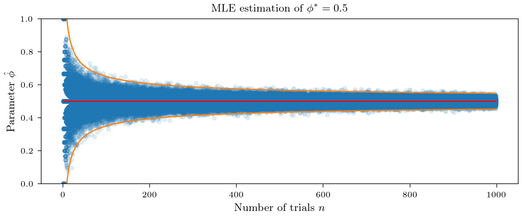
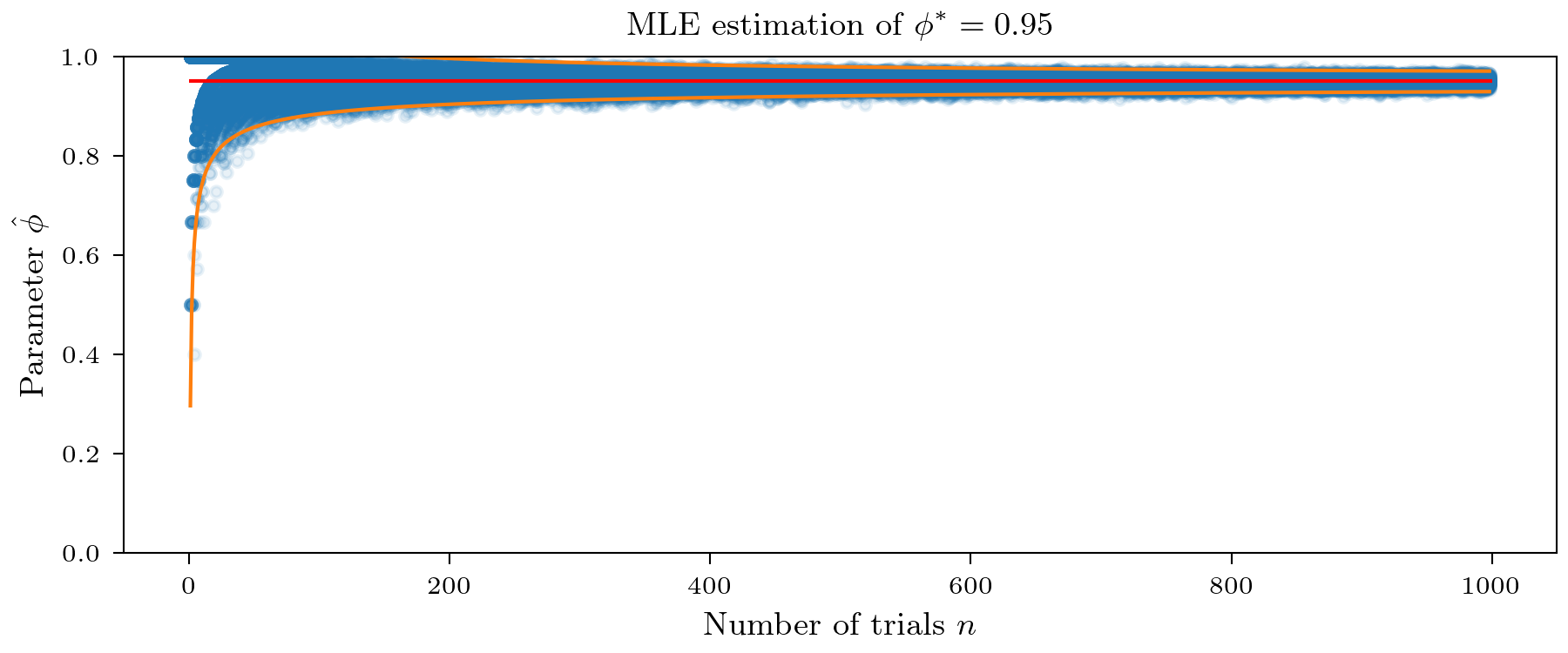
This also paves the way to approximate the sampling distribution of any MLE of an arbitrary statistical model. Note the sampling distribution of an MLE is the distribution of estimates given independent realizations $X_1, \dots, X_N \sim p_{\theta^*}$. For example for large enough $n$ MLE estimates will fall into the range \(\left( \theta^* - 2.96 \sigma_F, \theta^* + 2.96 \right)\) with (approximately) a $99%$ chance.

This is visually demonstrated in the figure below. Notice that even for small $n$ the approximation here is pretty good. Further as postulated by small Fisher information, it is harder to accurately estimate $\theta^* = 0.5$ than $\theta^*= 0.95$.

This allows us to construct a null hypothesis test for testing $\theta^* = \theta_0$. Let’s say we want to test

\[H_0: \theta^* = 0.5 \qquad H_1: \theta^* \neq 0.5\]

and choose an significance level of $\alpha = 0.01$. We know that for $n = 25$ trials, as a result $\sigma_F = 0.1$. Hence $99 \%$ of the time and MLE estimate would fall in between $(0.21, 0.79)$. Hence we would reject the null hypothesis if $\hat{\theta} < 0.21$ or $\hat{\theta} > 0.79$.

Constructing confidence intervals

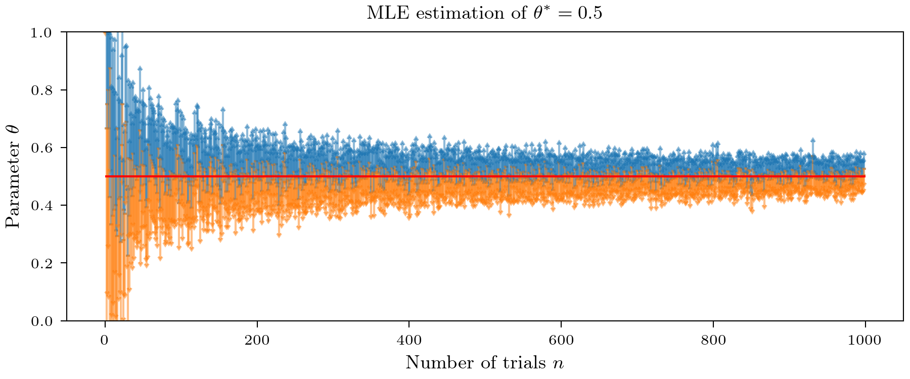
An alternative way to quantify our credibility in the estimate is to use confidence intervals. Recall that from the frequentist perspective the definition is a bit fuzzy: A $99\%$ confidence interval does not mean that the true value will lay in it with probability $0.99$ (this is called credible interval), but that if we estimate 100 such intervals that 99 of them will contain the true value. We can again just replace the true value with our estimate $\hat{\theta}$. This is visually demonstrated in the plot below.

FIM in Bayesian statistics

Until now we mostly discussed point estimates, so why is it also relevant in the Bayesian case? In the Bayesian paradigm, we start with existing prior beliefs about the parameter and update these beliefs based on information provided by data to guide inferential decisions.

Our prior beliefs are typically expressed in terms of a prior distribution $p(\theta)$, data is assumed to be generated by $p(x \mid \theta)$. Based on probability theory there is only a single way how observing $x$ should update our beliefs about our parameters, namely Baye’s theorem

\[p(\theta \mid x) = \frac{p(x \mid \theta)p(\theta)}{p(x)}\]

A clear connection to the frequentist approach is emerging as we delve into the use of point estimates derived from the full posterior distribution. While we could use methods like the posterior mean, variance, or mode, let’s strive to maintain a Bayesian perspective. This leads us to consider expanding the definition of the Fisher information matrix.

Given a generative model $p(x,\theta) = p(x|\theta)p(\theta)$. We define the Bayesian Fisher information matrix as $$ F = \mathbb{E}_{p(\theta)} \left[ F_x(\theta) \right] + \mathbb{E}_{p(\theta)} \left[\nabla_\theta \log p(\theta) \nabla_\theta \log p(\theta)^T \right]$$ here$ F_x(\theta)$ is the usual Fisher information as defined above.

Notice that in the Bayesian case, the Fisher information is constant for the parameter but does change concerning the prior. It is easy to see that as $p(\theta) \rightarrow \delta (\theta_0)$ (i.e. the prior becomes a point mass) also $F \rightarrow F_x(\theta_0)$ i.e. we recover the frequentist Fisher information evaluated at $\theta_0$.

The intuitive meaning also changes a bit. Given some $x \sim p(x)$ the BFIM can be seen as the amount of information $x$ carries averaged over any possible parameter, as specified by the prior plus the information provided by the prior itself. Similar to the frequentist case, the BFIM is connected to Bayesian parameter estimation and similar to the Cramer Rao lower bound, we can derive a lower bound for the variance of a Bayesian point estimator (van-Trees inequality). But I will not go into detail here.

Jeffrey priors

When performing Bayesian analysis, one of the crucial decisions is selecting a prior distribution that represents our prior beliefs about the parameters of interest. However, the choice of a prior can sometimes be subjective and lead to different conclusions, especially when the problem can be parameterized in various ways.

Imagine you’re dealing with a statistical problem where little is known about the parameter $\theta$ governing your data. In such cases, it may seem reasonable to assign a uniform prior distribution to $\theta$, essentially saying that no value of $\theta$ is favored over another. However, this approach can be problematic because the results may heavily depend on how the problem is parameterized.

To illustrate the challenges of the uniform prior, consider the example of a coin flip. When using a uniform prior on the coin’s propensity $\theta$, you might expect that it represents an unbiased belief. However, it turns out that this uniform prior can lead to different conclusions depending on how you parameterize the problem. For instance, if you parameterize the problem in terms of the coin’s angle $\eta$, a uniform prior on $\eta$ can yield highly informative priors on $\theta$. This lack of invariance raises questions about the reliability of the uniform prior as a default choice.

In order to obtain get a prior that is invariant to reparameterization of the problem, we can use the Jeffrey’s prior. It is defined as

\[p_{J}(\theta) = \frac{1}{Z} \sqrt{\det F_x(\theta)} \quad \text{with} \quad Z = \int \sqrt{\det F_x(\theta)} d\theta\]

We can now easily show that this prior is indeed invariant to reparameterization. Meaning that if we transform the parameter $\theta$ to $\eta$ the prior will remain the same!

(Jefreys prior invariance): Be $\theta$ and $\eta$ two parametrizations, related by a continuously differentiable function $\theta$ = f($\eta$). Then the Jeffrey's prior is invariant to reparameterization i.e. $$ p_{J}(\theta) = p_{J}(\eta) \det J_f(\eta) $$

[proof] Follows for reparameterization of the Fisher information matrix (see Lemma 2). We can write \(F_x(\eta) = J_f^T(\eta) F_x(\theta) J_f(\eta)\) thus we have \(\det F_x(\eta) = \det F_x(\theta) \cdot (\det J_f(\eta))**2\) and hence the statemant follows by plugging this into the definition of the Jeffrey’s prior. [/proof]

From this it also easily follows that any posterior distribution obtained using the Jeffrey’s prior is also invariant to reparameterization. This is a nice property as it ensures that the posterior distribution is independent of the parameterization of the problem.

Bayesian limit theorems

In the frequentist case, we saw that the MLE estimator is asymptotically normal. In the Bayesian case, we can also derive similar results. The first one is the Bernstein-von Mises theorem which states that the posterior distribution converges to a normal distribution with mean equal to the MLE and covariance equal to the inverse of the FIM.

(Bernstein-von Mises theorem): Be $X_1, \dots, X_n \sim p_{\theta^*}$. Assume that $p_{\theta^*}$ is well-specified, sufficiently regular and identifiable. Be $p(\theta)$ a prior distribution with support on a neighborhood of $\theta^*$. Then $$ p(\theta|x_1, \dots, x_n) = \mathcal{N}(\theta^*, \frac{1}{n} I(\theta^*)^{-1}) \quad \text{as} \quad n \rightarrow \infty$$

This does connect the Bayesian and frequentist approach. Note however that this result does only hold under relatively strict assumptions. These can be relaxed to a certain degree.

Conclusion

In essence, Fisher information is a fundamental concept that quantifies how much information data provides about model parameters, playing a central role in statistical analysis. As we saw this quantity just appears very often in a lot of different areas all over statistics.

References

[1] Alexander Ly, Maarten Marsman, Josine Verhagen, Raoul Grasman and Eric-Jan Wagenmakers (2017). A Tutorial on Fisher Information

[2] https://citeseerx.ist.psu.edu/viewdoc/download?doi=10.1.1.1037.2696&rep=rep1&type=pdf

[3] https://agustinus.kristia.de/techblog/2018/03/11/fisher-information/

[4] https://awni.github.io/intro-fisher-information/

[5] https://citeseerx.ist.psu.edu/viewdoc/download?doi=10.1.1.323.8983&rep=rep1&type=pdf